

Before comparing performance, it helps to understand the players. This post introduces the three main data-access techniques on an SAP HANA system: classic ABAP Open SQL, Core Data Services (CDS) views, and HANA Calculation Views. It covers what each one is, why it exists, and how they differ.
Ask three SAP developers how to read and aggregate data on a HANA system and you may get three different answers: “just write a SELECT,” “build a CDS view,” or “model it as a Calculation View.” All three are correct, and that is exactly what makes the topic confusing. Each technique comes from a different era and a different layer of the SAP stack, each has its own strengths, and each is consumed differently from ABAP.
This post walks through the three approaches one by one, then puts their differences side by side. It is the conceptual companion to our measured performance comparison; here the goal is understanding, not milliseconds.
Open SQL (in newer releases called simply ABAP SQL) is the SQL dialect built into the ABAP language. It is how ABAP programs have read database tables for decades:
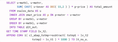
Its defining feature is database independence with deep ABAP integration. The same statement runs unchanged on any database SAP supports, because the ABAP kernel translates it into the native SQL of the underlying platform. Along the way, the kernel silently handles things the developer never has to think about: client handling (the MANDT filter is added automatically), type conversions between ABAP and database types, and efficient result transfer into internal tables.
Why is it used? Because it is the shortest path from an ABAP program to the data: no additional objects to create, no activation, no separate lifecycle. The query lives inside the program. Modern Open SQL has also grown powerful: joins, aggregations, CASE expressions, arithmetic inside SELECT lists, CTEs, and window functions are all available in current releases, which means substantial logic can be pushed down to the database in a single statement.
Its limitation is equally clear: an Open SQL statement is not reusable. The logic is trapped inside one program. If five reports need the same join-and-aggregate logic, it gets written five times, and that is precisely the problem the next technique solves.
Core Data Services (CDS) views are data models defined in Eclipse (ABAP Development Tools) as DDL sources. A CDS view captures a piece of data logic (joins, calculated fields, aggregations, associations) as a named, reusable, transportable object in the ABAP dictionary:
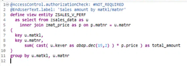
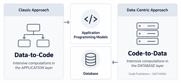
Any ABAP program can now consume this with a one-line SELECT, and every consumer gets the same, centrally maintained logic. Although the view is defined in the ABAP layer, it executes in the database. CDS is SAP’s primary vehicle for the code pushdown paradigm (“bring the code to the data”).
Compared with Open SQL, then, the difference is not where the query runs (both push down to HANA) but where the logic lives: inside one program versus as a shared, semantically rich dictionary object.
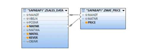
Calculation Views come from the other side of the fence: they are native HANA objects, created in the HANA Modeler (HANA Studio, or Web IDE / Business Application Studio in newer setups) rather than in the ABAP stack. Instead of writing code, the developer builds a graphical data flow: projection nodes to select and filter, join nodes, union nodes, aggregation nodes, star joins for dimensional models, and calculated columns for row-level expressions, ending in a semantics node that declares which fields are attributes and which are measures.
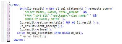
From ABAP, however, a Calculation View is a guest, not a family member. It follows the HANA repository’s own lifecycle and authorization concept (analytic privileges), and consuming it from ABAP requires a bridge: today typically ADBC (native SQL against the _SYS_BIC runtime object) or an AMDP table function wrapped in a CDS table function. The old Dictionary External View approach has been declared obsolete/deprecated; while it can still technically be created in some scenarios, its use is no longer recommended. Native SQL also means the conveniences of Open SQL, such as automatic client handling, no longer apply automatically.
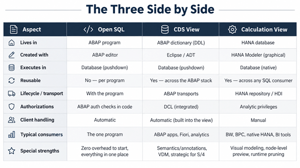
The honest answer: they are not competitors so much as tools for different homes. A quick decision guide:
Use Open SQL when the logic belongs to one program and reuse is not on the horizon. It is the simplest and most direct option, and with modern syntax it pushes down as much as the others.
Use CDS when the consumer is the ABAP world and the logic deserves to be a model: shared across programs, annotated for Fiori or analytics, secured with DCL, transported with the rest of the code. In S/4HANA this is the strategic default.
Use Calculation Views when you are working natively on HANA (BW/BPC scenarios, cross-schema models, database-level transformations) or when the graphical, node-by-node development style genuinely fits the problem.
And performance? All three execute in the database, so the old intuition “closer to the database = faster” no longer separates them cleanly. Whether they actually perform identically on the same workload is an empirical question, and answering it properly, with measurements, traces, and execution plans, is exactly what we did in the companion post to this one. The short version: the results were not what the textbook ordering predicts.

SAP Fiori Consultant
Emrah Tezcan, who serves as an SAP ABAP & Fiori Consultant at MDP Group, is a highly skilled SAP expert developing enterprise solutions based on ABAP Cloud and the RAP (RESTful ABAP Programming Model) on the S/4HANA architecture. With deep expertise in extensibility approaches aligned with the Clean Core strategy, HANA Output Management, Adobe Forms, and Flexible Workflow processes, Tezcan takes end-to-end responsibility across the entire software development lifecycle (SDLC), from analysis and design to testing/UAT, go-live, and post-production support.
Your mail has been sent successfully. You will be contacted as soon as possible.
Your message could not be delivered! Please try again later.